Cart-Pole Problem Revisited: Trajectory Optimisation and more

Problem statement: Given a cart carrying a pole attached to it at the centre by a rotary joint, the challenge is to keep the pole vertical only using the motion of the cart, i.e. the only variable under our control is the force given to the cart at each instant. The number of variables required to describe a given configuration of the system entirely is 2, the position of the cart and the angle of the pole measure from the vertical in the anti-clockwise direction. But the variables we can control is 1, hence an under-actuated system.

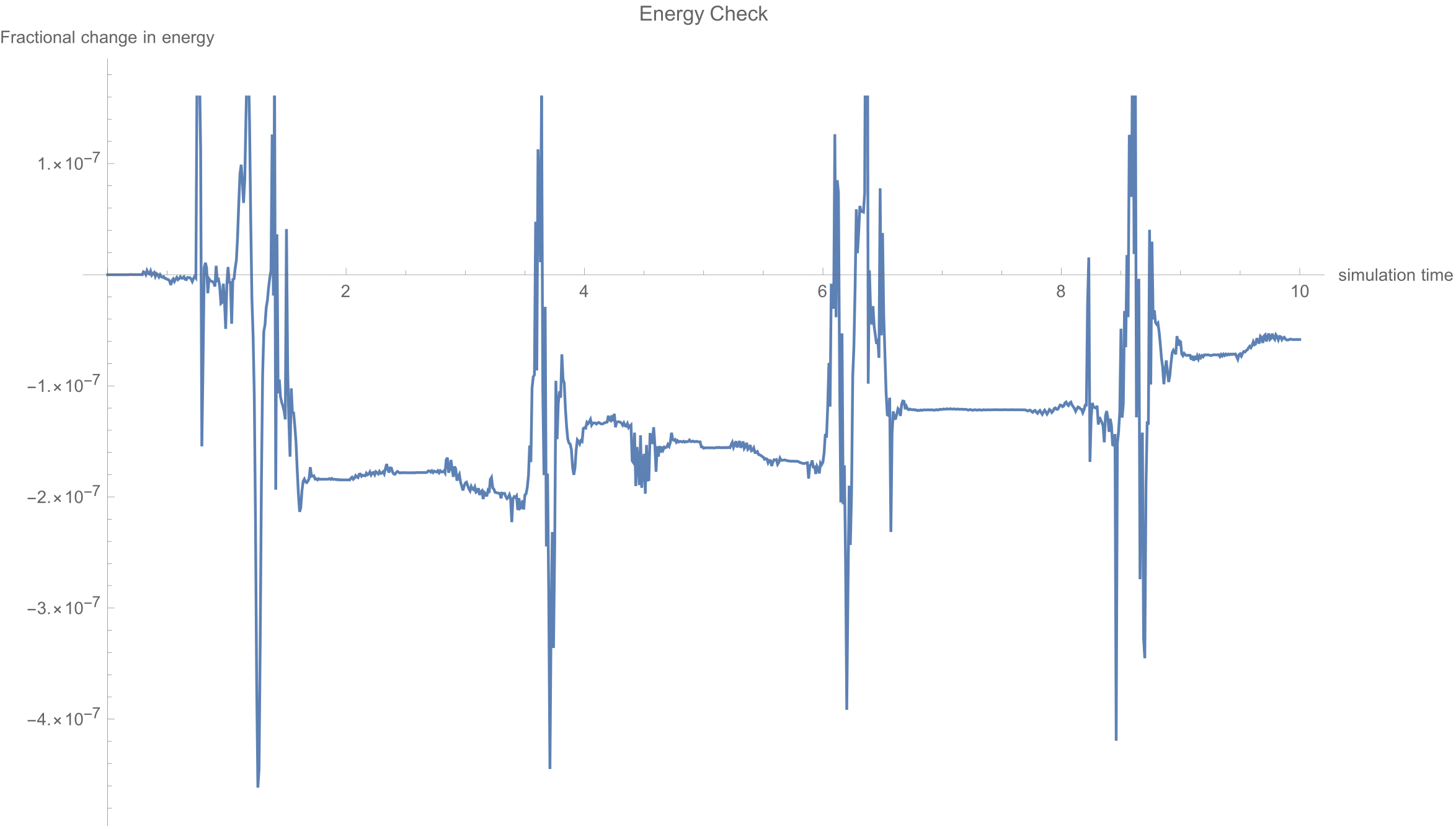
The dynamics of the system is derived using Euler-Lagrange formulation and then converted into state-space representation, which is of the form xdot = f(x), where x is the vector of generalised coordinates(x1 = cart position and x2 = angle of the pole, x3 = velocity of the cart and x4 = angular velocity of the pole). One way to validate the mathematical model is to check the percentage change in the total energy of the system as it evolves from a given initial condition without external forces.

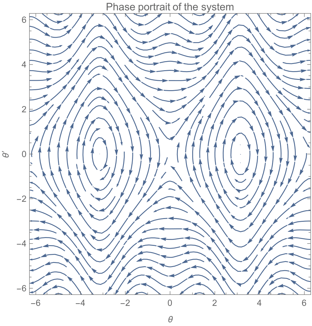
Setting f(x) to 0 gives us the equilibrium set, which is x1 can be any number whereas x2 = 0, pi, -pi, x3=0, x4=0. The configuration x2 = +-pi represent the unstable equilibrium point as seen from the phase portrait of x2, x4.

Now we try out different controllers which take the pole and stabilises it at its unstable equilibrium position.

Task-1: Design a full state feedback controller.

1. Linearise the system about the unstable equilibrium point, xdot = A.x+b.u.
2. Let the control input be of the from u=Kx, where x is the full state vector. 3.Construct the modified A’ matrix, A’ = (A-bk).
3. Get the characteristic polynomial of A’ and get the conditions of stability using the Rouths criteria.
4. Tune the gains k1, k2, k3, k4 satisfying these conditions and also satisfy to meet the performance requirements.
5. Simulate the non-linear system using the controller obtained from a linear model.

Task-2: Design a Linear Quadratic Regulator(LQR). Seeing the controller effort required in the previous case, we would want to solve this problem by using smaller efforts. So we put a constraint on the effort in this case.

1. Same linear model as above.
2. We get the gain as K = -R^-1.B^T.P
3. Assuming the existence of an asymptotic solution, we set Pdot = 0 and solve the Riccati equation for P.
4. Tune the values of Q and R to satisfy performance conditions.

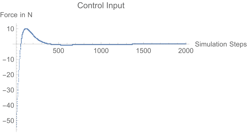
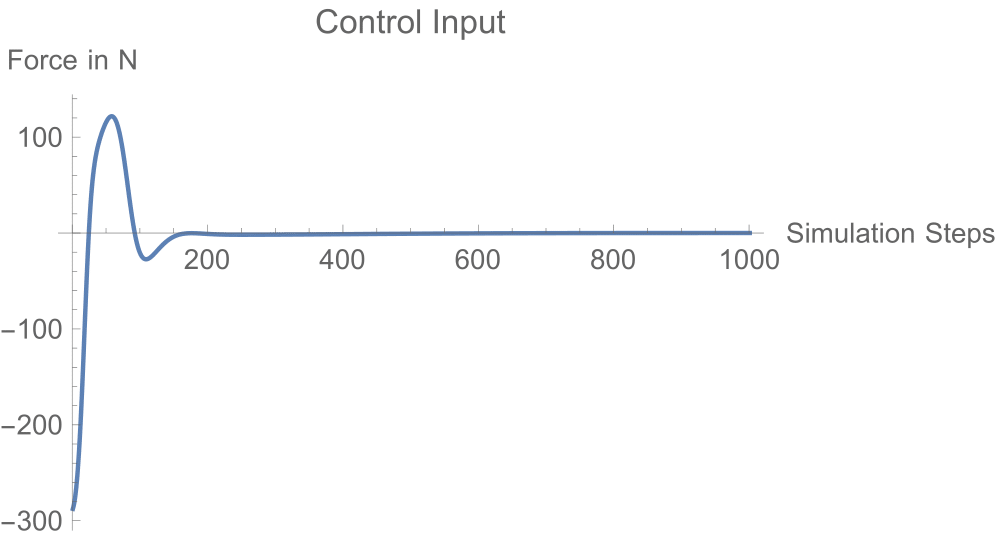
What we have done until now is to obtain a controller from the linearised model and use it to control the non-linear system. We see that in both cases, the controllers are still capable of stabilising errors as huge as 60 degrees. So why even bother about non-linear system analysis if this works just fine?

Task-3: Energy Shaping

Let’s have a look again at the phase-portrait of the pendulum.

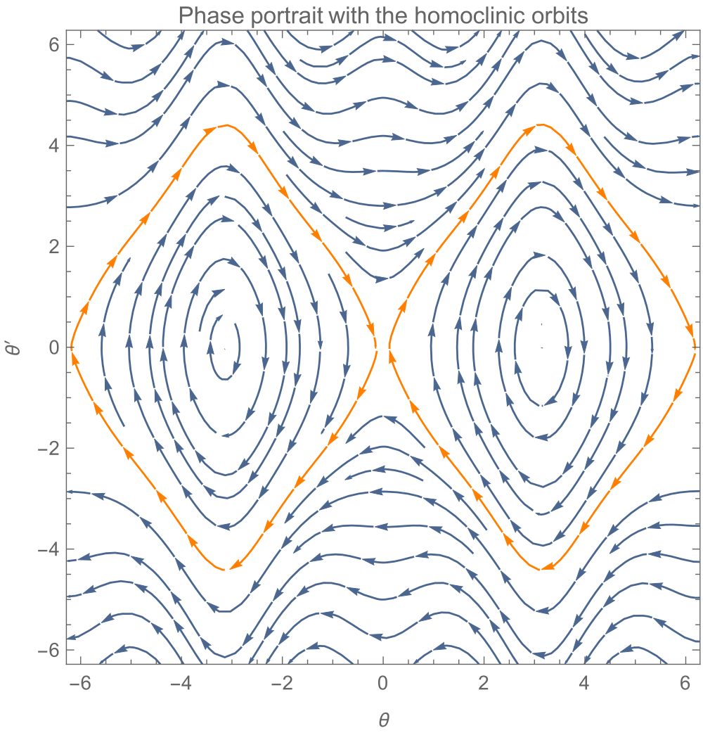
Have a closer look at the point through which the orange orbit passes

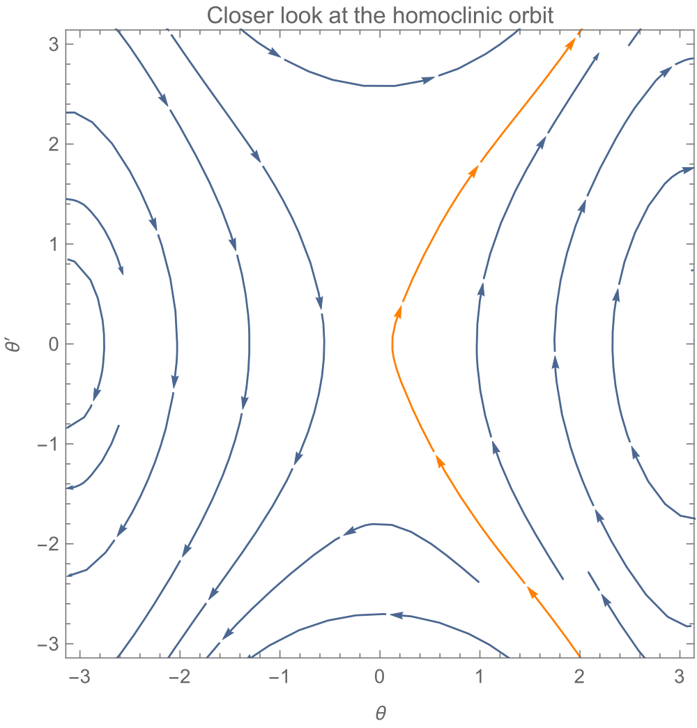
(Though it looks like a continuous orbit, in reality as we go closer to origin the lines terminates and originates from it).

Starting at any point on the orange orbit would automatically (evolves without any external control) take the system to the unstable equilibrium point (0,0). So given an initial configuration, it is enough if we steer the system until it hits this orbit. This is the essence of this control strategy. For more information refer to this textbook.

As seen, the controller takes the system to the orange orbit, which drives the system to the unstable equilibrium point. The path taken by the system (dotted red line) and the phase portrait of the modified system after the application of control is as shown.

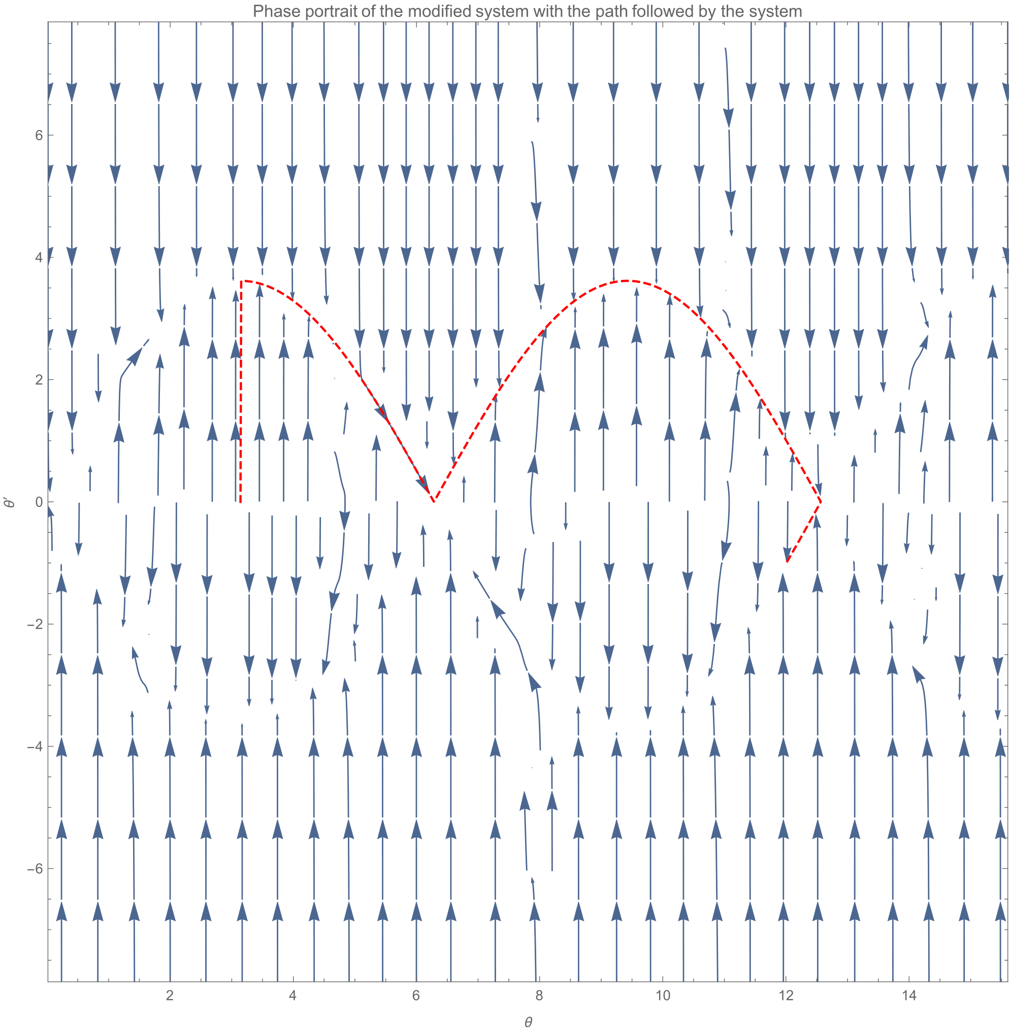
Interesting point is that, if there are any numerical errors in the states, these small deviations in its configuration drives the system along the orbit until it comes back to the unstable state again. This tells us that this is not a stabilising controller.

Task-4: Trajectory Optimisation

When we cannot come up with a controller, we can obtain the required control input by discretising the system and posing the problem as an optimisation problem, with the system, state and actuator constraints.

A beautiful introductory tutorial on this topic can be found here.

In our case, we have 80 discretised states and the objective is to minimise the net control input.

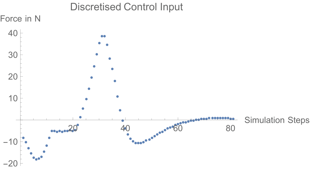
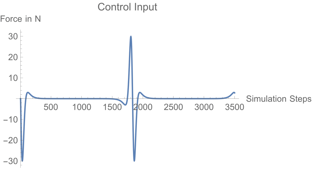
Discussion: Coming to the question of why one has to study non-linear control; the control input plots clearly show a trend. The controllers arising from a linear model assumption drive the system through the entire time and have larger absolute magnitudes. Whereas the non-linear controllers exploit the system dynamics to get the job done cutting down the efforts.

All the codes are available in this GitHub repository.